Statistical shape and appearance modelling with pyssam

This statistical shape and appearance modelling example visualises modes of shape and appearance correlations in the left lower lung lobe. Appearance values are obtained from the gray-value at the pixel nearest to each landmark on a digitally reconstructed radiograph (DRR) that mimics a frontal (anterior-posterior) chest X-ray. DRRs are created from the patient CT image data by integrating the voxel intensity over a chosen direction. We done this using the script in ZacharAdn/ct_2_xRay.

import pyssam

from copy import copy
from glob import glob
import matplotlib.pyplot as plt
import numpy as np

First, we source landmark data to use in our shape model

LANDMARK_DIR = "../../example_data/lung_landmarks/"
XR_DIR = "../../example_data/reconstructed_xrays/"
# Get directories for DRR and landmark data
origin_dir_list = glob(f"{XR_DIR}/origins/origins/drr*.md")
spacing_dir_list = glob(f"{XR_DIR}/*/drr*.md")
im_dir_list = glob(f"{XR_DIR}/*/drr*.png")
origin_dir_list.sort()
spacing_dir_list.sort()
im_dir_list.sort()
# check that user has declared correct directory
patientIDs = [i.split("/")[-1].replace(".png", "")[-4:] for i in im_dir_list]
landmark_dir_list = glob(f"{LANDMARK_DIR}/landmarks*.csv")
landmark_dir_list = sorted(
  landmark_dir_list, key=lambda x: int(x.replace(".csv", "")[-4:])
)
# used to align drrs and landmarks
trans_dirs = glob(f"{XR_DIR}/transforms/transformParams_case*_m_*.dat")
trans_dirs.sort()

if (
  len(im_dir_list) == 0
  or len(origin_dir_list) == 0
  or len(landmark_dir_list) == 0
  or len(spacing_dir_list) == 0
):
  raise AssertionError(
    "ERROR: The directories you have declared are empty.",
    "\nPlease check your input arguments.",
  )

landmark_offset = np.vstack(
  [np.loadtxt(t, skiprows=1, max_rows=1) for t in trans_dirs]
)
# read data
origin = np.vstack([np.loadtxt(o, skiprows=1) for o in origin_dir_list])
spacing = np.vstack([np.loadtxt(o, skiprows=1) for o in spacing_dir_list])
# load x-rays into a stacked array,
# switch so shape is (num patients, x pixel, y pixel)
img_all = np.rollaxis(np.dstack([pyssam.utils.loadXR(o) for o in im_dir_list]), 2, 0)
landmark_coordinates = np.array(
  [np.loadtxt(l, delimiter=",") for l in landmark_dir_list]
)

# offset centered coordinates to same reference frame as CT data
landmark_align_to_projection = (
  landmark_coordinates + landmark_offset[:, np.newaxis]
)

from pyssam.utils import AppearanceFromXray
appearance_helper = AppearanceFromXray(
    img_all,
    origin[:, [0, 2]],
    spacing[:, [0, 2]]
)
appearance_scaled = appearance_helper.all_landmark_density(landmark_align_to_projection[:, :, [0, 2]])

using 2D coordinates for X-ray

Initialising the model

Here we convert to landmark coordinates into a parameterised shape model. We first initialise the class, which handles all pre-processing. Then, we can compute the shape model components and mean population shape

ssam_obj = pyssam.SSAM(landmark_coordinates, appearance_scaled)
ssam_obj.create_pca_model(ssam_obj.shape_appearance_columns)
mean_shape_appearance_columnvector = ssam_obj.compute_dataset_mean()

Plotting and analysis

# Define some plotting functions

def plot_cumulative_variance(explained_variance, target_variance=-1):
    number_of_components = np.arange(0, len(explained_variance))+1
    fig, ax = plt.subplots(1,1)
    color = "blue"
    ax.plot(number_of_components, explained_variance*100.0, marker="o", ms=2, color=color, mec=color, mfc=color)
    if target_variance > 0.0:
        ax.axhline(target_variance*100.0)

    ax.set_ylabel("Variance [%]")
    ax.set_xlabel("Number of components")
    ax.grid(axis="x")
    plt.show()

def plot_ssam_modes(
  mean_shape_appearance_columnvector,
  original_shape_parameter_vector,
  shape_model_components,
  show_difference=True,
  mode_to_plot=0,
):
  print(f"explained variance is {ssam_obj.pca_object.explained_variance_ratio_[mode_to_plot]}")

  weights = [-2, 0, 2]
  fig, ax = plt.subplots(1, 3)
  for j, weights_i in enumerate(weights):
    shape_parameter_vector = copy(original_shape_parameter_vector)
    shape_parameter_vector[mode_to_plot] = weights_i
    mode_i_morphed = ssam_obj.morph_model(
        mean_shape_appearance_columnvector,
        shape_model_components,
        shape_parameter_vector
    ).reshape(-1, 4)
    mean_appearance_columnvector = mean_shape_appearance_columnvector.reshape(-1, 4)[:, 3]
    mode_i_appearance = mode_i_morphed[:, 3]

    offset_appearance = (mean_appearance_columnvector - mode_i_appearance)
    if weights_i != 0 and show_difference:
      ax[j].scatter(
        mode_i_morphed[:, 0],
        mode_i_morphed[:, 2],
        c=offset_appearance,
        cmap="seismic",
        vmin=-1,
        vmax=1,
        s=1,
      )
    else:
        ax[j].scatter(
        mode_i_morphed[:, 0],
        mode_i_morphed[:, 2],
        c=mode_i_appearance,
        cmap="gray",
        s=1,
        )
    if weights_i == 0:
        ax[j].set_title("mean shape")
    else:
        ax[j].set_title(f"mode {mode_to_plot} \nweight {weights_i}")

    ax[j].axis('off')
    ax[j].margins(0,0)
    ax[j].xaxis.set_major_locator(plt.NullLocator())
    ax[j].yaxis.set_major_locator(plt.NullLocator())

  plt.show()

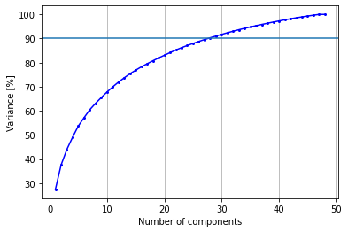
Generally, the first part in assessing the model once trained is visualising how the explained variance changes with an increasing number of modes. If few modes are required, it means it will be much simpler to fit the SSM to an image.

print(f"To obtain {ssam_obj.desired_variance*100}% variance, {ssam_obj.required_mode_number} modes are required")
plot_cumulative_variance(np.cumsum(ssam_obj.pca_object.explained_variance_ratio_), 0.9)

To obtain 90.0% variance, 27 modes are required

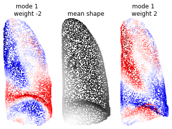
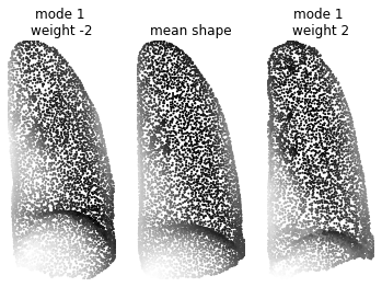
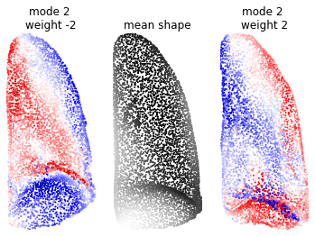
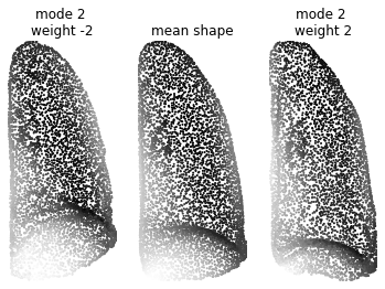
Now the interesting part. We visualise the first three principal components, where the points are coloured by their displacement.

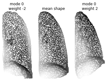
mode_to_plot = 0

plot_ssam_modes(
    mean_shape_appearance_columnvector,
    ssam_obj.model_parameters,
    ssam_obj.pca_model_components,
    mode_to_plot=mode_to_plot,
)
plot_ssam_modes(
    mean_shape_appearance_columnvector,
    ssam_obj.model_parameters,
    ssam_obj.pca_model_components,
    show_difference=False,
    mode_to_plot=mode_to_plot,
)

explained variance is 0.2740360637188665

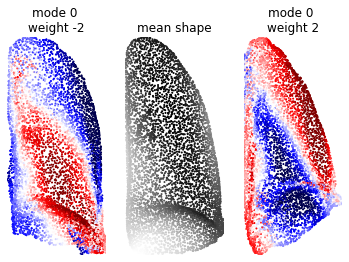
explained variance is 0.2740360637188665

mode_to_plot = 1

plot_ssam_modes(
    mean_shape_appearance_columnvector,
    ssam_obj.model_parameters,
    ssam_obj.pca_model_components,
    mode_to_plot=mode_to_plot,
)
plot_ssam_modes(
    mean_shape_appearance_columnvector,
    ssam_obj.model_parameters,
    ssam_obj.pca_model_components,
    show_difference=False,
    mode_to_plot=mode_to_plot,
)

explained variance is 0.10199336940057746

explained variance is 0.10199336940057746

mode_to_plot = 2

plot_ssam_modes(
    mean_shape_appearance_columnvector,
    ssam_obj.model_parameters,
    ssam_obj.pca_model_components,
    mode_to_plot=mode_to_plot,
)
plot_ssam_modes(
    mean_shape_appearance_columnvector,
    ssam_obj.model_parameters,
    ssam_obj.pca_model_components,
    show_difference=False,
    mode_to_plot=mode_to_plot,
)

explained variance is 0.06396590938304687

explained variance is 0.06396590938304687

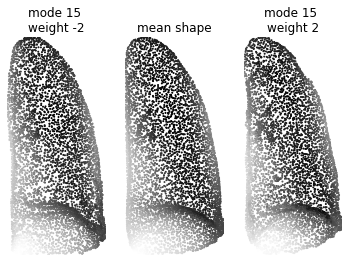
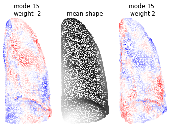
When we look at the 15th mode, which accounts for around 1% for the total variance, we can see a very minor change in the lung structure (shown by very light red and blue patches).

mode_to_plot = 15

plot_ssam_modes(
    mean_shape_appearance_columnvector,
    ssam_obj.model_parameters,
    ssam_obj.pca_model_components,
    mode_to_plot=mode_to_plot,
)
plot_ssam_modes(
    mean_shape_appearance_columnvector,
    ssam_obj.model_parameters,
    ssam_obj.pca_model_components,
    show_difference=False,
    mode_to_plot=mode_to_plot,
)

explained variance is 0.014082077705233292

explained variance is 0.014082077705233292