Mesh morphing with pyssam
This example visualises how pyssam can be used to visualise SSM modes of variance as a surface.
On this dataset, and definitely more real-world datasets, the results of the morphing will be highly dependent on the quality of the template. If the results are not satisfactory, simply use a template which is more similar to the target.
[1]:
import pyssam
[2]:
from copy import copy
import matplotlib.pyplot as plt
import numpy as np
import vedo as v
First, we source landmark data to use in our shape model
[3]:
N_SAMPLES = 50
torus = pyssam.datasets.Torus()
torus_data = torus.make_dataset(N_SAMPLES)
landmark_coordinates = np.array([torus_i.points() for torus_i in torus_data])
Initialising the model
Here we convert to landmark coordinates into a parameterised shape model. We first initialise the class, which handles all pre-processing. Then, we can compute the shape model components and mean population shape
[4]:
# if USE_SCALED_DATA = True, we should have 1 mode. If False, we should have 2 modes.
USE_SCALED_DATA = True

ssm_obj = pyssam.SSM(landmark_coordinates)
if USE_SCALED_DATA:
    ssm_obj.create_pca_model(ssm_obj.landmarks_columns_scale)
else:
    ssm_obj.create_pca_model(landmark_coordinates.reshape(N_SAMPLES, -1))
mean_shape_columnvector = ssm_obj.compute_dataset_mean(ssm_obj.landmarks_columns_scale)
mean_shape = mean_shape_columnvector.reshape(-1, 3)
shape_model_components = ssm_obj.pca_model_components
/Users/josh.williams/gitrepos/pyssam-loadmodel/pyssam/statistical_model_base.py:269: UserWarning: Dataset mean should be 0, is equal to [-2.40707919e-07  1.30819524e-08  1.12504786e-07 -8.63408829e-08
 -6.27933687e-08 -1.54367029e-07 -2.72104614e-07  1.20353960e-07
 -2.93035725e-07 -2.82570170e-07  4.70950283e-08  1.54367029e-07
  8.89572718e-08 -4.00307727e-07  3.13966844e-08 -6.27933687e-08
 -8.11081051e-08 -1.17737571e-07  1.17737571e-07  1.36052307e-07
  1.98845669e-07  1.56983422e-08  4.44786359e-08 -4.97114172e-08
  1.85763724e-07 -9.15736678e-08  1.98845669e-07  5.75605910e-08
  4.44786359e-08 -2.72104614e-07  4.68333894e-07  1.04655618e-08
  2.09311235e-08  2.48557086e-07 -3.13966865e-07  6.01769798e-08
  2.09311235e-08  0.00000000e+00 -4.18622470e-08  5.75605910e-08
  1.20353960e-07 -8.11081051e-08 -3.45363532e-07  1.22970349e-07
  4.44786359e-08 -4.55251950e-07  1.54367029e-07  2.98268503e-07
  6.54097576e-08  1.33435918e-07]
  warn("Dataset mean should be 0, " f"is equal to {dataset.mean(axis=1)}")
Plotting and analysis
[5]:
# Define some plotting functions

def plot_cumulative_variance(explained_variance, target_variance=-1):
    number_of_components = np.arange(0, len(explained_variance))+1
    fig, ax = plt.subplots(1,1)
    color = "blue"
    ax.plot(number_of_components, explained_variance*100.0, marker="o", ms=2, color=color, mec=color, mfc=color)
    if target_variance > 0.0:
        ax.axhline(target_variance*100.0)

    ax.set_ylabel("Variance [%]")
    ax.set_xlabel("Number of components")
    ax.grid(axis="x")
    plt.show()

def plot_shape_modes(
  mean_shape_columnvector,
  mean_shape,
  original_shape_parameter_vector,
  shape_model_components,
  mode_to_plot,
):
  weights = [-2, 0, 2]
  fig, ax = plt.subplots(1, 3, figsize=(10, 4))
  x_min, x_max, y_min, y_max = np.inf, -np.inf, np.inf, -np.inf
  mode_outputs = []
  for j, weights_i in enumerate(weights):
    shape_parameter_vector = copy(original_shape_parameter_vector)
    shape_parameter_vector[mode_to_plot] = weights_i
    mode_i_coords = ssm_obj.morph_model(
        shape_parameter_vector
    ).reshape(-1, 3)
    print(mode_i_coords.min(axis=0), mode_i_coords.max(axis=0))

    offset_dist = pyssam.utils.euclidean_distance(
      mean_shape,
      mode_i_coords
    )
    # colour points blue if closer to point cloud centre than mean shape
    mean_shape_dist_from_centre = pyssam.utils.euclidean_distance(
      mean_shape,
      np.zeros(3),
    )
    mode_i_dist_from_centre = pyssam.utils.euclidean_distance(
      mode_i_coords,
      np.zeros(3),
    )
    offset_dist = np.where(
        mode_i_dist_from_centre<mean_shape_dist_from_centre,
        offset_dist*-1,
        offset_dist,
    )
    if weights_i == 0:
      ax[j].scatter(
        mode_i_coords[:, 0],
        mode_i_coords[:, 1],
        c="gray",
        s=1,
      )
      ax[j].set_title("mean shape")
    else:
      ax[j].scatter(
        mode_i_coords[:, 0],
        mode_i_coords[:, 1],
        c=offset_dist,
        cmap="seismic",
        vmin=-1,
        vmax=1,
        s=1,
      )
      ax[j].set_title(f"mode {mode_to_plot} \nweight {weights_i}")
    mode_outputs.append(mode_i_coords)
    if mode_i_coords[:,0].min() < x_min:
        x_min = mode_i_coords[:,0].min()
    if mode_i_coords[:,1].min() < y_min:
        y_min = mode_i_coords[:,1].min()
    if mode_i_coords[:,0].max() > x_max:
        x_max = mode_i_coords[:,0].max()
    if mode_i_coords[:,1].max() > y_max:
        y_max = mode_i_coords[:,1].max()
    ax[j].axis('off')
    ax[j].margins(0,0)
    ax[j].xaxis.set_major_locator(plt.NullLocator())
    ax[j].yaxis.set_major_locator(plt.NullLocator())

  for j, weights_i in enumerate(weights):
    ax[j].set_xlim([x_min, x_max])
    ax[j].set_ylim([y_min, y_max])
  plt.show()
  return mode_outputs
To check how different the shapes we are dealing with are, we first visualise the modes as point cloud from pyssam.
[6]:
mode_to_plot = 0
print(f"explained variance is {ssm_obj.pca_object.explained_variance_ratio_[mode_to_plot]}")

mode_outputs = plot_shape_modes(
    mean_shape_columnvector,
    mean_shape,
    ssm_obj.model_parameters,
    ssm_obj.pca_model_components,
    mode_to_plot,
)
explained variance is 0.9926544427871704
[-2.47113479 -2.48272705 -1.16445051] [2.47113479 2.45901084 1.16445051]
[-2.29824519 -2.31162167 -0.79496741] [2.29824519 2.28437424 0.79496741]
[-2.12535559 -2.14051628 -0.42548432] [2.12535559 2.10974027 0.42548432]

If the variable USE_SCALED_DATA above is true, the following should show essentially no variation.
[7]:
mode_to_plot = 1
print(f"explained variance is {ssm_obj.pca_object.explained_variance_ratio_[mode_to_plot]}")

plot_shape_modes(
    mean_shape_columnvector,
    mean_shape,
    ssm_obj.model_parameters,
    ssm_obj.pca_model_components,
    mode_to_plot,
)
explained variance is 0.00734558142721653
[-2.34566274 -2.35931855 -0.81101496] [2.34566274 2.33150221 0.81101496]
[-2.29824519 -2.31162167 -0.79496741] [2.29824519 2.28437424 0.79496741]
[-2.25082764 -2.26392479 -0.77891987] [2.25082764 2.23725036 0.77891987]

[7]:
[array([[-3.58806753e-05,  2.33149812e+00, -1.57952403e-09],
        [ 3.55803679e-10,  2.31845573e+00,  1.44958303e-01],
        [ 4.08452689e-10,  2.27973549e+00,  2.85257430e-01],
        ...,
        [ 3.30136920e-10,  2.27973549e+00, -2.85257434e-01],
        [ 3.30128386e-10,  2.31845573e+00, -1.44958293e-01],
        [ 3.30127967e-10,  2.33150221e+00, -1.58371696e-09]]),
 array([[ 3.23460236e-09,  2.28437424e+00,  6.36053044e-10],
        [ 3.23460236e-09,  2.27158594e+00,  1.42090023e-01],
        [ 3.23460236e-09,  2.23363185e+00,  2.79613048e-01],
        ...,
        [ 3.23456595e-09,  2.23363185e+00, -2.79613048e-01],
        [ 3.23456506e-09,  2.27158594e+00, -1.42090008e-01],
        [ 3.23456439e-09,  2.28437424e+00,  6.36052711e-10]]),
 array([[ 3.58871445e-05,  2.23725036e+00,  2.85163012e-09],
        [ 6.11340105e-09,  2.22471615e+00,  1.39221743e-01],
        [ 6.06075204e-09,  2.18752821e+00,  2.73968666e-01],
        ...,
        [ 6.13899498e-09,  2.18752821e+00, -2.73968662e-01],
        [ 6.13900173e-09,  2.22471615e+00, -1.39221723e-01],
        [ 6.13900082e-09,  2.23724626e+00,  2.85582238e-09]])]
The above plots are useful, but it is nicer to visualise the output as a surface.
Mesh morphing
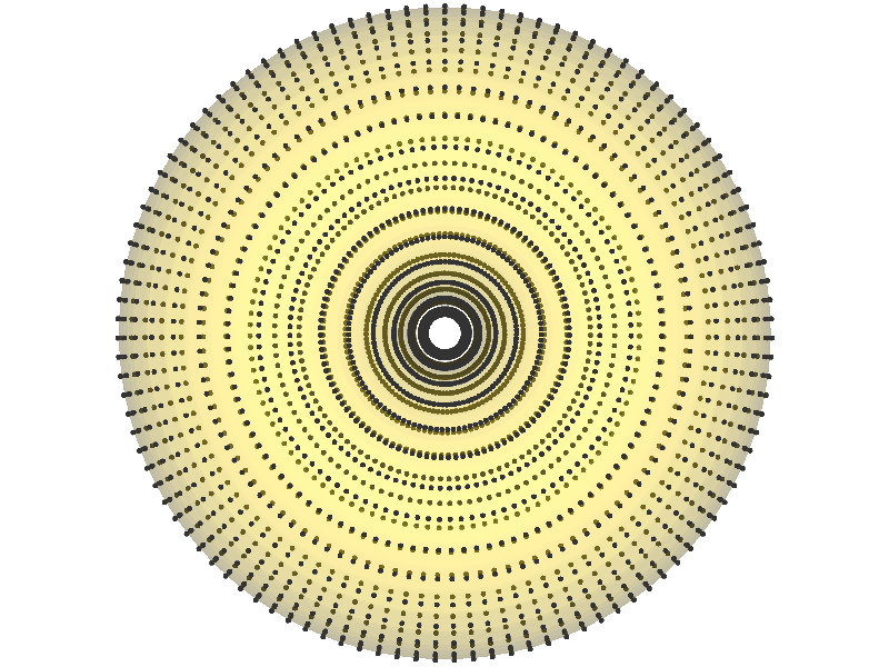
First, lets look at the template mesh and template landmarks (blue). We also show the target landmarks as black for comparison.
[8]:
TEMPLATE_CASE = 0
landmark_target = mode_outputs[0]
mesh_template = torus_data[TEMPLATE_CASE]
landmark_template = landmark_coordinates[TEMPLATE_CASE]
v.show(mesh_template.alpha(0.2), v.Points(landmark_template, r=5, c="blue"), v.Points(landmark_target, r=5))

Now we will mesh the template to the target. We then will visualise the target mesh and landmarks.
[9]:
mesh_target_i = pyssam.morph_mesh.MorphTemplateMesh(landmark_target, landmark_coordinates[TEMPLATE_CASE], torus_data[TEMPLATE_CASE]).mesh_target
v.show(mesh_target_i.alpha(0.2), v.Points(landmark_target, r=5))